Box User Manual (0.2.0)
| Authors: | Matteo Franchin |
|---|---|
| Licence: | GNU Lesser General Public License (LGPL) version 3 |
| Version: | 0.3.0 compiled 2011-10-22 at 22:10. |
| Home page: | http://boxc.sourceforge.net |
Outline of document
Introduction
Box is an object oriented programming language which allows you to easily draw figures.
Installation
There are currently three methods for installing Box:
- Installation from sources: can be done easily on Unix platforms (Linux, Mac OS) and somewhat less easily on Microsoft Windows platforms;
- Installation on Ubuntu Linux: can be done easily downloading the deb package and using dpkg -i;
- Installation on Windows: just a matter of downloading a zip archive. The executable can be used immediately after unzipping the archive.
Installation from sources
Download the tarball from http://sourceforge.net/projects/boxc. This is usually a file with name such as box-0.1.tar.gz. Then untar and configure the package with:
tar xzvf box-0.1.tar.gz
cd box-0.1
./configure --prefix=/usr
configure outputs a summary at the end. Be sure it looks like that:
Configuration summary:
----------------------
Support for the Cairo 2D graphic library: yes
If you get a "no" then check that the Cairo graphics library http://www.cairographics.org is installed on your system together with the development files. On Ubuntu and Debian derivatives, you can install it with:
sudo aptitude install libcairo libcairo-dev
You should enter the root password when necessary for the installation to proceed. If you were required to install Cairo, then reconfigure the package with ./configure --prefix=/usr. You can then proceed to the compilation with:
make
If the compilation is succesful:
sudo make install
The Box executable, libraries and headers will be installed on your system. You can take a look at the man page with:
man box
Further help and hints with the installation can be found on the README and INSTALL files inside the package.
The manual is online at http://boxc.sourceforge.net. If you need further help, take a look at the examples.
Note for installation on Mac OS
If you compiled Box from source on Mac OS and you experience problems when loading libraries (-l g seems not to work as it should), try to reconfigure Box with the additional option --with-included-ltdl, such as:
./configure --prefix=/usr --with-included-ltdl
and then compile it again. This should force the use of the provided ltdl (libtool) library and should fix the bug.
Installation on Ubuntu Linux
Download the Ubuntu package from http://sourceforge.net/projects/boxc. This is usually a file with name such as box_0.1-0ubuntu1_i386.deb. Install it with:
sudo dpkg -i box_0.1-0ubuntu1_i386.deb
Enter the root password when necessary. You may have to install libcairo with:
sudo aptitude install libcairo
This is often not necessary, as Cairo is usually preinstalled on an average Ubuntu distribution.
The manual is online at http://boxc.sourceforge.net. If you need further help, take a look at the examples.
Installation on Windows
Download the zip file from http://sourceforge.net/projects/boxc. This is usually a file with name such as box20080727.zip. Unzip it inside the directory which is more convenient for your needs. You'll find the Box executable in box20080727\bin\box.exe and some examples inside box20080727\examples. Make a check as follows: open the MS-DOS prompt and enter the examples directory:
cd box20080727\examples
..\bin\box.exe translucency.box -l g
You can then view the produced output file translucency.png with your favourite image viewer. As an alternative, to run a Box source file, you can just right click on the file icon and select "Open with...". Then browse the directory where you unzipped the binaries: select the file box-lg.bat under the directory box20080727\bin which was created when unzipping the Box binaries (box-lg.bat is equivalent to box.exe -l g). Proceed and open the file (tick on "Remember application" if you want Windows to use Box automatically when double clicking on Box sources). The file should be executed immediately and the output images should be generated, if any.
Remember that the directory box20080727 can be moved to another location, this won't affect the functionality of Box. However you have to move the whole directory, preserving its structure: the box executable searches for libraries and headers in the directory DIR\..\lib\box, where DIR is the directory which contains the executable box.exe.
The manual is online at http://boxc.sourceforge.net. If you need further help, take a look at the provided examples.
Command reference
PointList
The PointList instruction can be used to create an array of named points. The typical use is:
pl = PointList["name1", point1, "name2", point2, ...]
The name is optional and, if given, comes just before the point it refers to. Here is an example:
// Create a PointList object containing 3 points
pl = PointList["one", (10, 20), "two", (50, 50), (100, 50)]
The points can be retrieved using the Get method:
// You can refer to points by index and by name!
p1 = pl.Get[1]     // The points of pl can be retrieved by index...
p2 = pl.Get["two"] // ...or by name
p2 = pl.Get[3]     // The third point can only be referred by index, since
                   // we didn't provide a name!

// You can iterate over the points with:
i = 1, Print[pl.Get[i], For[++i <= pl.Num[]];] // Print all the points of pl
The last line shows how you can iterate over the elements of pl. n = pl.Num[] is the number of points in the PointList, which is just 3 in the above example. The elements are numbered starting from 1. You can however use indices outside the interval 1 - n:
// Ciclic indexing!
last = pl.Get[4]         // Returns the first point, which is pl.Get[1]
last = pl.Get[0]         // Returns the last point, which is pl.Get[3]
last = pl.Get[-1]        // Returns the second last point, which is pl.Get[2]

// You can use floating point indices!
middle_12 = pl.Get[1.5]  // The point centered between pl.Get[1] and pl.Get[2]
near_1 = pl.Get[1.1]     // This point is quite near to pl.Get[1]
near_2 = pl.Get[1.9]     // and this is quite near to pl.Get[2]
pl.Get[0] returns the last element of the list (the one returned also by pl.Get[n], where n = pl.Num[]) and, in general, indices differing by a multiple of n refer to the same element (circular indexing). The method Get can take also a real number as an argument: if pl.Get[1] gives the first point of the list and pl.Get[2] gives the second, then pl.Get[1.5] gives the point in the middle of these. Mathematically, if x is a positive number less than unity: pl.Get[i+x] == pl.Get[i] + x*(pl.Get[i+1] - pl.Get[i]), for every integer number i. As a further extension, the Get method can take also a point as an argument.
// You can use even a Point index!!!
x = 1.234
between_12 = pl.Get[(x, 0)] // This is equivalent to...
between_12 = pl.Get[x]      // ...this. For every x!

p = pl.Get[(1.6, 0.7)]      // The y component moves the point orthogonal
                            // to the current segment.
// p could be calculated also as:
v = pl.Get[2] - pl.Get[1]      // The vector "containing" 1.6
o = (-v.y, v.x)                // The orthogonal vector
p = pl.Get[1] + 0.6*v + 0.7*o  // But this is somewhat more complicated :-)
The y component of the point index corresponds to the direction orthogonal to the one of the x component. The example above shows how the point index is used to compute the point returned by the method Get. Notice that there are two ways to choose a vector orthogonal to a given one (in 2 dimensions). Here we adopt the convention o = (-v.y, v.x).
Extending an existing PointList is very simple:
Print[pl;] // Print the PointList object
\ pl[(200, 50), "hey!", (123, 456)] // pl can be extended easily
Print[pl;] // Now pl has 5 elements!
Further points are added to the PointList by just reopening pl. Here is the output of the previous lines:
Color instruction
The Color instruction can be used to create colors. It is a structure composed by four real numbers (Real r, g, b, a). The members r, g and b correspond respectively to the red, green and blue components of the color, while the a member is the alpha channel and can be used to define translucent (transparent) colors. These real number can be set to values which range from 0.0 to 1.0, corresponding respectively to lowest and highest intensity. When the alpha channel is set to 0 the color is fully transparent when set to 1 the color is fully opaque. A new color can be defined using the following syntax:
color = Color[.r=0.1, .g=0.2, .b=0.3, .a=0.4]
Colors can be defined starting from existing colors:
red = Color[.a=.r=1.0, .g=.b=0.0]    // define the opaque red
transparent_red = Color[red, .a=0.5] // copy red and change the alpha channel
The header file "g" defines a structure which contains some predefined colors:
color = (Color black, red, green, yellow, blue, magenta, cyan, white
         dark_red, dark_green, dark_yellow, dark_blue, dark_magenta
         dark_cyan, grey, none)
You can set the current color in drawing instructions such as Poly, Circle, etc.
\ w.Poly[..., color, ...]
or directly inside an opened window:
w = Window[][ ..., color, ...]
Gradient
Gradient is used to create color gradients to be used when filling.
Window
Window objects play the central role in the graphic library. Indeed, every graphic command has a Window as a target. There are many types of windows, all of them however fall in one of three cathegories:
- bitmap windows: windows of this type draw into memory. The image surface is reduced to a grid of pixels. The color of each pixel is stored into an allocated region of the memory of your computer. The content of such a window can be saved into a PNG file.
- stream (vector) windows: a window of this type is associated to a file. Any graphic command induces new data to be appended to this file.
- recoder windows: a window which simply records the commands, so that they can be re-used and manipulated in a later stage.
The minimal commands to create a window are:
w = Window[]                                    // for a recorder window
w = Window["rgb24", (100, 50)]                  // for a bitmap window
w = Window["pdf", (100, 50), .File["file.pdf"]] // for a pdf stream window
The window type is identified by a string. If the user does not provide a string, then a recorder window will be created by default ("fig" is the string associated to recorder windows). Here is a list of available window types, together with their identificative string:
| cathegory | id string | window type | requires |
| bitmap | "a1" | alpha channel (1 bit per pixel) | Cairo |
| "a8" | alpha channel (8 bit per pixel) | ||
| "rgb24" | RGB (24 bit per pixel) | ||
| "argb32" | RGB + alpha channel | ||
| stream | "pdf" | Output to PDF file | |
| "svg" | Output to SVG file | ||
| "cairo:eps" | Output to EPS file | ||
| "eps" | Output to EPS file | Native | |
| record | "fig" | Commands are recorded |
Most of these windows are available only when the graphic library is compiled with support for the Cairo 2D graphics library. Window[] takes also the following arguments:
- the size of the window: compulsory for bitmap and stream windows. It is expressed in millimeters, i.e. (100, 50) corresponds to a window with 100 mm width and 50 mm height.
- the name of the output file. This is required only when creating stream windows. Example: w = Window[.File["name.ext"], ...].
- the resolution. This is meaningful only for bitmap windows and specifies the number of pixels per millimeter in both x and y direction. Example: w = Window[.Res[Dpi[400]], ...]. Here the function Dpi converts the resolution from points per inch (dpi) to points per mm.
- the origin. Example: If the window is created with w = Window[(sx, sy), .Origin[(ox, oy)]], then the it will show the points (px, py) with px between ox and ox + |sx| and py between oy and oy + |sy|. Here |sx| and |sy| are the absolute values of sx and sy respectively. The sign of sx and sy is used to mirror the window along the correspondent direction.
We emphasize that all the numbers used in graphics commands are expressed in millimeters (mm). If you prefer to use inches, you should scale your figure before saving it.
Note: most of the times the user may just want to use a record window ("fig") and save its content to file with the Window.Save method. This method takes care of calculating the bounding box of the figure you want to save. It allows to save just the portion of your drawing which is actually visible and chooses a different target by looking at the extension of the provided output file.
Incomplete windows
Incomplete windows are created when the user does not provide all the parameters which are necessary for the creation of a window. For instance:
w = Window["rgb24"]
Here the size of the window is not being specified, but there won't be complains and w will be created as an incomplete window. An error message will however be displayed as soon as the user tries to draw something inside it. Incomplete windows can be used together with the method Window.Save, which is discussed below.
Window.Save
This method is useful only for bitmap windows and for record windows.
for bitmap windows this method offers a way to transfer the image, which is currently stored in the RAM memory of your computer, into a PNG file (only PNG is supported as an output image format). Here is an example:
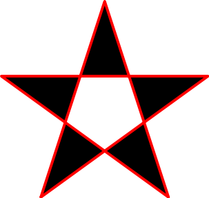
// Create a bitmap window and save it.
w = Window["rgb24", (50, 50), .Origin[(-25, -25)], .Res[Dpi[100]]]
s = Style[.Border[1, color.red]] // Just to trace a red border
i = 0, \ w.Poly[40*Vec[Deg[18+i*144]], For[++i < 5], s] // a star
w.Save["html/window1.png"]
The output of this small fragment of code is shown below:

Notice that a part of the picture lies outside the visible region: the star tips are cut.
for record windows this method allows to transfer the recorded commands to a new or existing window. Here is an example:
w2 = Window[] // create a recorder window
i = 0, \ w2.Poly[40*Vec[Deg[18+i*144]], For[++i < 5], s]
w2.Save["html/window2.png"]
Only the file name needs to be provided to the Save method: the size is computed automatically and is large enough to contain the picture. The extension of the given file name is used to decide what kind of output format to use. In this case "argb32" (the default) is used to create a temporary target window, whose content is then saved to the given file, using PNG as an image format. The output is:
The picture recorded inside w2 can be used again to create, for example, an EPS and a SVG file with:
w2.Save["html/window2.eps"]
w2.Save["html/window2.svg"]
The Window.Save method however is much more flexible than what you may think at this point. For example, you may want to use "rgb24", instead of "argb32". This is the situation where Incomplete windows become handy:
w2.Save["html/window3.png", Window["rgb24", .Res[Dpi[50]]]]
This line specifies to use a resolution of 50 dpi (points per inch) and "rgb24" as the intermediate bitmap format. This is the image you get:

The w2.Save method uses the provided window as follows:
If the provided window is incomplete, then it is completed, computing the bounding box of w2 and using it as a size for the output window. We say that the provided incomplete window is completed. Indeed, after the method has been called the window becomes usable:
w3 = Window["rgb24"]    // w3 is incomplete
                        // Here w3 cannot be used
w2.Save["file.png", w3] // w3 iw completed
w3.Circle[(0, 0), 20]   // w3 is now a normal window and can be used!
This does two things: put the content of w2'' inside ``w3'' and put the same content inside a file ``"file.png". You can avoid the latter, if you just omit the file name:
w2.Save[w3] // w3 iw completed and no file is saved to disk
If you provide a normal window (complete window), then w2 is scaled to fit in it, before actually being put in it.
Window.Hot
The Window.Hot method is used to insert a new point into the list of hot points of a window. This method is used in conjunction with Window.Put.
Window.Put
The Put instruction can be used to transform and place figures into other figures.
Style
Style can be used to set the filling styles for polygons and all the other shapes. It can be used to set the filling scheme, the border width, dash pattern, join and cap styles.
Window.Poly
The Poly method can be used to draw polygons. It takes a list of points with optional margins:
point_list = window.Poly[first_margin0, second_margin0, point1,
                         first_margin1, second_margin1, point2,
                         first_margin2, second_margin2, point3, ...]
The margins are real numbers and are used for rounding the corners. You can omit them, if you want to draw a polygon with sharp corners. For instance:
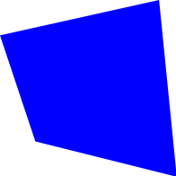
a = (5, 40), b = (50, 50),  c = (55, 0),  d = (15, 10)
pl = w.Poly[color.blue, a, b, c, d]
draws a polygon with vertices a, b, c and d. This is the produced output:
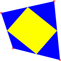
The Poly instruction returns a PointList object containing the vertices of the polygon. This PointList can be used in many ways. It can be used, for example, to draw the polygon which connects the mid-points of the original polygon sides:
i = 1, \ w.Poly[color.yellow, pl.Get[i+0.5], For[++i < 5]]
\ w.Circle[Color[color.red, .a=0.5], 1, pl] // Circles on vertices
To understand the first line, you should take a look at the documentation for the PointList object. Here we just remind that pl.Get[1.5] is the point between pl.Get[1] and pl.Get[2]: the point at the center of the first side of the polygon. The second line here draws transparent red circles with radius 1 and center on the points of the PointList pl. Note that here we use \ to ignore the PointList expression generated by the Poly method invocation. This is the result:
Now we focus on how the polygon corners are rounded. The idea is the following: for every edge of the polygon we identify a sub-segment, which is just a part of it. All the sub-segments are then traced one after the other, using ellipse arcs to connect them. In practice, between the vertices p1 and p2 of the polygon, you can specify two real numbers r1 and r2:
\ w.Poly[..., p1, r1, r2, p2, ...]
The optional numbers r1 and r2 are used to specify which part of the edge p1-p2 has to be connected with a straight line. All the remaining bits are rounded! In particular r1 specifies the first margin, i.e. the distance between the first point of the edge p1 and the first point of the sub-segment m1. r2 specifies the second margin, i.e. the distance between the second point of the sub-segment m2 and the second point of the edge p2. They are calculated as m1 = p1 + r1*(p2 - p1) and m2 = p2 + r2*(p1 - p2). Consequently when r1 = r2 = 0 for all the edges, the polygon corners are not rounded (this is the default behaviour). When r1 = r2 = 0.5 the polygon is "fully rounded", meaning that it is made just of ellipse arcs. It should be clear now that r1 and r2 must be positive numbers whose sum can't be greater than 1. If this is not the case, then the value new_r1 = Max[0.0, Min[1.0, r1]] is used for the first margin, while for the second, Max[0.0, Min[new_r1, r2]] is used. Here is an example:
\ w.Poly[color.yellow
         a, 0, 0.05, b, 0.1, 0.15, c, 0.2, 0.5, d, 0.2, 0]
which gives:
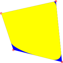
Note that it is not necessary to specify both the margins: if just the first margin r1 is given, the second is assumed to be the same (r2 = r1). This behaviour makes sense only when r1 <= 0.5 (remember that r1 + r2 has to be lower than 1.0). Therefore, when r1 > 0.5, r2 is calculated as 1.0 - r1. If both the margins are not given, then the old margins are used. In particular:
Poly[..., p1, r1, r2, p2, p3, p4, ...]
is equivalent to:
Poly[..., p1, r1, r2, p2, r2, r1, p3, r1, r2, p4, ...]
Note that the old margins are used with reversed order! This behaviour makes it easy to draw corners with equal margins.
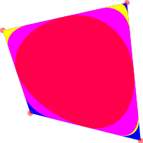
A single Window.Poly instruction can be used to draw several polygons, using the ; separator. Here is an example:
\ w[Style[.Fill[";"]]]
\ w.Poly[color.magenta, 0.2, pl;
         Color[color.red, .a=0.7], 0.5, pl]
Notice that we used the PointList object, which we obtained previously. We also set the drawing style for the window w. This is necessary because a Poly instruction can be used also to draw polygons with holes. This is actually the default drawing style: polygons separated by ; in the same Poly instruction are used to draw just one figure with holes (the inner polygon is the hole). We use Style[.Fill[";"]] to avoid this behaviour and force the Poly instruction to start to draw a different polygon whenever ; is found (see the documentation of the Style object for more info). Here is the result:
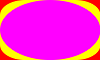
The rounding procedure works such that, if rect is a PointList containing the vertices of a rectangle, .Poly[0.5, rect] draws the corresponding ellipse. Here is an example:
rect = w2.Poly[color.red, (0, 0), (50, 0), (50, 30), (0, 30)] // a rectangle
\ w2.Poly[color.yellow, 0.25, rect] // partial rounding
\ w2.Poly[color.magenta, 0.5, rect] // full rounding makes it an ellipse!
which gives:
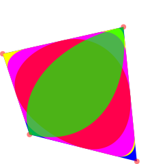
With margins greater than 0.5:
\ w.Poly[Color[color.green, .a=0.7], 0, 1, pl]
we obtain:
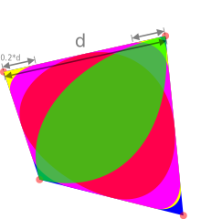
The PointList returned by the Poly instruction can be used to do other fancy things:
// Rulers
\ w.Line[Color[color.black, .a=0.5], 0.4, h=0.03
         arrow_ruler, pl.Get[(1, -h)], arrow_ruler, pl.Get[(1.999, -h)];
         arrow_ruler, pl.Get[(1, h)], arrow_ruler, pl.Get[(1.2, h)];
         arrow_ruler, pl.Get[(1.8, h)], arrow_ruler, pl.Get[(1.999, h)]]

// Labels
w.Text[.Font["Sans", 5], pl.Get[1.5], .From[(1, -0.5)], "d";
       .Font["Sans", 2], pl.Get[1.1], .From[(1, -1.2)], "0.2*d"]
and here is the result:
Here is the Box code used to generate all the pictures in this subsection:
include "g"
include "arrows"

w = Window[]

// Draw one plain polygon
a = (5, 40), b = (50, 50),  c = (55, 0),  d = (15, 10)
pl = w.Poly[color.blue, a, b, c, d]
w.Save["html/poly1.png"]

// Draw another polygon from the mid-points of the edges of the original one
i = 1, \ w.Poly[color.yellow, pl.Get[i+0.5], For[++i < 5]]
\ w.Circle[Color[color.red, .a=0.5], 1, pl] // Circles on vertices
w.Save["html/poly2.png"]

\ w.Poly[color.yellow
         a, 0, 0.05, b, 0.1, 0.15, c, 0.2, 0.5, d, 0.2, 0]
w.Save["html/poly3.png"]

\ w[Style[.Fill[";"]]]
\ w.Poly[color.magenta, 0.2, pl;
         Color[color.red, .a=0.7], 0.5, pl]
w.Save["html/poly4.png"]

\ w.Poly[Color[color.green, .a=0.7], 0, 1, pl]
w.Save["html/poly5.png"]

w2 = Window[]
rect = w2.Poly[color.red, (0, 0), (50, 0), (50, 30), (0, 30)] // a rectangle
\ w2.Poly[color.yellow, 0.25, rect] // partial rounding
\ w2.Poly[color.magenta, 0.5, rect] // full rounding makes it an ellipse!
w2.Save["html/ellipse.png"]

// Rulers
\ w.Line[Color[color.black, .a=0.5], 0.4, h=0.03
         arrow_ruler, pl.Get[(1, -h)], arrow_ruler, pl.Get[(1.999, -h)];
         arrow_ruler, pl.Get[(1, h)], arrow_ruler, pl.Get[(1.2, h)];
         arrow_ruler, pl.Get[(1.8, h)], arrow_ruler, pl.Get[(1.999, h)]]

// Labels
w.Text[.Font["Sans", 5], pl.Get[1.5], .From[(1, -0.5)], "d";
       .Font["Sans", 2], pl.Get[1.1], .From[(1, -1.2)], "0.2*d"]

w.Save["html/poly6.png"]
Window.Circle
Circle can be used to draw circles, ellipses and rings. Its syntax is:
window.Circle[center1, radius1_x, radius1_y;
              center2, radius2_x, radius2_y; ...]
center1, center2 the centers (Point objects) of the circles/ellipses, radius1_x, radius2_x, radius1_y, radius2_y are the radii (Real numbers).
Window.Text
The Text instruction can be used to write text.
Window.Line
The Line instruction can be used to lines width variable width. It takes a list of points with optional line width:
point_list = window.Line[point1, initial_width1, final_width1
                         point2, initial_width2, final_width2
                         ...]
The widths are real numbers and are used to specify what the line widths are when entering and exiting each point of the line. initial_width is the width when exiting from point1, while final_width1 is the width when entering point2. You can omit them, if you want to draw a line with constant width.
The line in the following picture,
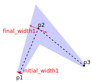
was obtained using:
\ w.Line[p1, 3, 10, p2, 15, 2, p3]
The Window.Line instruction does also accept Color and Style objects to set the color and the filling/border style of the line. It does also accept LineStyle objects, which are used to control how the smoothing is done.
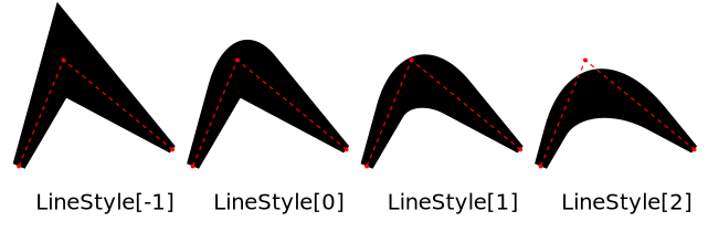
The lines in the image above were obtained using:
\ w.Line[LineStyle[x], p1, 3, 10, p2, 15, 2, p3]
For x = -1, 0, 1 and 2.
How are version numbers stuck over Box?
We adopt two version regimes. The young regime and the mature regime. In the young regime, the version string is composed by three numbers MAJOR.MINOR.PATCH. PATCH is increased just for bug fixes or for extensions of the language that are compatible with the previous version. MINOR is increased when the new release is not compatible with the previous one. MAJOR will be increased to end the young regime and enter into the mature regime. Notice that the three parts of the version MAJOR, MINOR and PATCH are integer numbers and can be greater than 9. Different versions of Box can coexist, but only when they differ in their MINOR or MAJOR part of the version. The idea here is that one always wants to replace a previous version of the Box compiler, with a newer one, if this is just a patch. For this reason the directories created inside lib/ and include/ have the form boxMAJOR.MINOR and the PATCH part is omitted. The Box core library has the name libboxcoreMAJOR.MINOR.so.CUR.REV.AGE meaning that each incompatible release of Box will have a different independent library. Releases just differing for the PATCH part have the same core library name and therefore the CUR.REV.AGE part should be handled with care (this is done automatically by box/admin/version.sh). Regarding the mature regime, we are not defining here rigid rules. We anticipate that probably compatibility will be regarded as a more important issue in the mature regime. We indeed intend to pass to the mature regime only when the number of Box users will be big enough to limit our freedom of changing the language, hoping that this will really happen, soon or later...